The 1990 National Science Teachers Association (NSTA) publication of Science Teachers Speak Out: The NSTA Lead Paper on Science and Technology Education for the 21st Century called for educators to develop and implement science curricula that integrate appropriate technology and make science learning more efficient and effective through computers. In addition, the NSTA (1999) has further contended that “computers should have a major role in the teaching and learning of science” (Rationale, ¶ 1).
Standards have been proposed by leading national science education organizations for the integration of technology into science classrooms and for the preparation of science teachers (Flick & Bell, 2000), which include the following:
- Technology should be introduced in the context of science content.
- Technology should address worthwhile science with appropriate pedagogy.
- Technology instruction in science should take advantage of the unique features of technology.
- Technology should make scientific views more accessible.
- Technology instruction should develop understanding of the relationship between technology and science. (p. 40)
Similar standards were proposed for the preparation of mathematics teachers (Garofalo, Drier, Harper, Timmerman, & Shockey, 2000):
- Introduce technology in context.
- Address worthwhile mathematics with appropriate technology.
- Take advantage of technology.
- Connect mathematics topics.
- Incorporate multiple representations. (p. 66)
These guidelines are not only appropriate for the use of technology in the preparation of science and mathematics teachers, they are also relevant to the use of technology in all science and mathematics disciplines. A general “rule of thumb” is that technology should be used in the teaching and learning of science and mathematics when it allows one to perform investigations that either would not be possible or would not be as effective without its use. Although several technologies meeting these criteria for instructional use are available for physics instruction, some educators are still “struggling with whether technology refers only to calculators and computers or to a much wider range of potential instructional aids” (Lederman & Niess, 2000, p. 345).
Technology Examples
According to Mottmann (1999), two of the more important reasons for introducing technology and other instructional innovations into physics education are “1) to improve students’ physics ability, and 2) to improve students’ negative reactions toward physics” (p. 75). Rios and Madhavan (2000) identified four classifications of technologies that are appropriate for physics instruction and provided brief descriptions of a few examples. The classifications were (a) computer interfacing equipment to collect and process data, (b) experimental or theoretical modeling, (c) computer simulations requiring graphics, and (d) research/reference/presentation programs for gathering, reporting, and/or displaying information. The following is an updated and expanded description and discussion of several forms of technology fitting into each of these categories that physics educators should find to be most successful in facilitating improved understandings of physics concepts. Also included is selected research related to the use of each.
Computer Interfacing Equipment to Collect and Process Data
Figures 1a & 1b. Calculator-Based Ranger (CBR) screen shots.
Some of the more common interfacing devices are probes that plug into graphing calculators or computers. According to the NSTA (1999), “Microcomputer Based Laboratory Devices (MBL’s) should be used to permit students to collect and analyze data as scientists do, and perform observations over long periods of time enabling experiments that otherwise would be impractical” (Declarations, ¶ 3). Available probes commonly used in physics activities include timers, force scales, “sonic rangers,” thermometers, light and sound meters, and probes serving as electrical multimeters. Students can quickly and efficiently gather data from the probes and then display it graphically and/or enter it into a spreadsheet program for further manipulation. The “major advantage of using interfacing equipment is the time saved when students no longer have to perform repetitive observations in which they learn no new skills” (Rios & Madhavan, 2000, p. 94). The use of this type of technology allows students to have more time to perform repeated data collection trials and for conceptual analysis of the experimental data.
The most widely used probes include products available from scientific supply vendors such as PASCO, Vernier, and Texas Instruments. Figure 1 shows sample results of one-dimensional motion displayed on the TI 83+ graphing calculator screen that were obtained using a Texas Instruments Calculator-Based Ranger (CBR). Cost, functionality, and compatibility comparisons of several of these products are available from Rios and Madvavan (2000), although their descriptions may now be dated.
Research indicates that the use of sensors/probes is effective, particularly in the area of graphical interpretation. “Brasell (1987) and Thorton and Sokoloff (1990) found that students using real-time graphs with MBL significantly improved their kinematics graphing skills and their understanding of the qualitative aspects of motion they observed, compared to students using delay-time graphs” (Escalada & Zollman, 1997, p. 469). An early study by Beichner (1990) found that students taught with MBLs achieved more success than did students taught by simulations and demonstrations, although significant improvements in computer simulations since the study may lead to different results today. Although Brungardt and Zollman (1995) found no significant differences between learning with real-time and delay-time analysis, they did notice that students using MBLs appeared to be more motivated and demonstrated more discussion in their groups.
Experimental or Theoretical Modeling
Exercises in modeling offer students “an idea of how a real physicist works in determining equations that fit the study being made” (Rios & Madhavan, 2000, p. 95). Although mathematical models are probably the most common type of model used in physics, models can also be concrete physical representations, verbal analogies, static or dynamic visual representations, and combinations of each of these.
Because most physics concepts and interactions can be easily modeled with mathematical relationships, computer generated models of these relationships are found in virtually all areas of physics. An electrical modeling program “in which students explicitly construct, evaluate, revise, and improve their model of electricity” (Steinberg & Wainwright, 1993, p. 357) has shown both achievement gains and increased confidence as a result of the program. The study also found that confidence levels of female students had the most significant increase as a result of this program.
Some computer models seek to greatly simplify the situation being modeled (conceptual models), while others seek to represent the situation being modeled as realistically as possible (phenomenological models). Figure 2 displays a screen shot of a dynamic Web-based conceptual model for charging an electroscope that is linked to the Ross Sheppard Physics Web site, http://www.shep.net/resources/curricular/physics/P30/Unit2/electroscope.html. This use of “plus” (+) and “minus” (-) signs to represent charged objects and/or charged regions of an object is common when attempting to have students develop an understanding of electrostatics.
Figure 2. Conceptual model of electroscope charging.
Otero, Johnson, and Goldberg (1999) advocated the use of both phenomenological and conceptual models in carefully designed learning sequences. Although there may be many forms of models, “the purpose for which any model is originally produced in science is as a simplification of the phenomenon to be used in enquiries to develop explanations of it” (Gilbert, Boulter, & Elmer 2000, p. 11). Among items that Graham and Rowlands (1998) listed as “primary advantages of using computer software in the development of mental models” (p. 483) are considerations related to the detail of information provided, time management, reproducibility of experimentation, ability to vary experimental parameters, and analysis capabilities. The ability to model dynamic events with dynamic models is also an important capability of computer generated models.
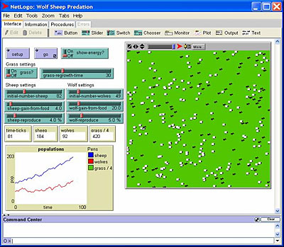
Figure 3. NetLogo screen shot.
Although most computer simulations,especially those found on the Web, offer no student manipulation of the assumptions behind the models, some software programs allow students to build their own models and program in a variety of assumptions. One such program, NetLogo, allows users to program complex dynamic models of systems interactions with virtually no limit to the number and type of assumptions to guide the model (Figure 3).
Another popular modeling program is STELLA. Like NetLogo, STELLA allows the user to construct dynamic models of systems interactions. Each of these is an excellent program for modeling cause-and-effect relationships and interactions and can be effectively used for some physics applications. However, they may not be considered the best choice available for modeling introductory level physics phenomena, due to the complexity of the programming required.
In contrast, Interactive Physics (Figure 4) is a commercially available program designed especially for physics modeling that is being increasingly used across the United States in introductory high school and university physics courses. A modeling program such as Interactive Physics “is an environment in which almost any physical situation can be recreated and monitored” (Graham & Rowlands, 2000, p. 486) and can “provide excellent visual images in conjunction with numerical, graphical or vector representations of different quantities” (p. 489). This program has been used in modeling forces associated with both static and dynamic situations and has been shown to attain “excellent agreement between the real and simulated systems” (Hasson & Bug, 1995, p. 235). Many other modeling programs currently exist, and one can assume that more will continue to be developed with increasing sophistication and ease of use.
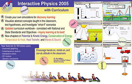
Figure 4. Interactive Physics
One type of technological innovation that could be considered a “hybrid” between computer interfacing/data collection equipment and modeling software would be digital video analysis programs (Bryan, 2005). The video camera is used to “collect” position and time data, which can then be used to mathematically and graphically model anything related to the position and/or motion of the object. By using digital video’s frame advance features and “marking” the position of a moving object in each frame, students are able to determine more precisely the position of an object at much smaller time increments than would be possible with common timing devices such as photo gates, stopwatches, or mechanical “dot timers.” Once the student collects data consisting of positions and times, these values may be manipulated for determinations of velocity and acceleration, and if mass is known, other values such as kinetic and potential energies, force, momentum, etc. Students may then graphically display their collected and calculated data and insert these graphs and information into other documents.
Several relatively inexpensive commercially available video analysis programs such as VideoPoint, Physics ToolKit (formerly known as World-in-Motion), and Measurement-in-Motion are currently gaining widespread use in physics instructional settings. Vernier has also added video analysis capabilities in the latest version of their LoggerPro software. Other programs are also becoming available for no cost (e.g., DataPoint and Tracker). These programs serve as an effective means to both collect, analyze, and report data and make possible the analysis of some situations that would not otherwise be possible. For example, an analysis of the kinetic and potential energies associated with a bouncing ball make it possible to examine the energy conservation as the ball rises and falls after each bounce and also examine the loss of total mechanical energy during each bounce (Bryan, 2004). Video of an object revolving around an external point allows the user to readily examine both rotational and linear motion.
Six important advantages of video analysis over MBL probes and sensors are that a) video analysis allows study of two-dimensional motion, like a revolving object or projectiles, b) video analysis has no distance limitations, c) more than one object can be analyzed in a video, leading to detailed comparisons of objects that are in the same system, d) video analysis can be performed without all of the cumbersome wires and sensors, e) most video analysis programs enable the user to examine multiple representations of the phenomena (note the detailed graphical, tabular, mathematical, and pictorial motion representations displayed “side by side” in the same full screen computer window (Figure 5) in contrast to the single small sketchy displays generated using the “sonic ranger” in Figure 1, and f) anything captured on film – past, present, or future – may be analyzed.
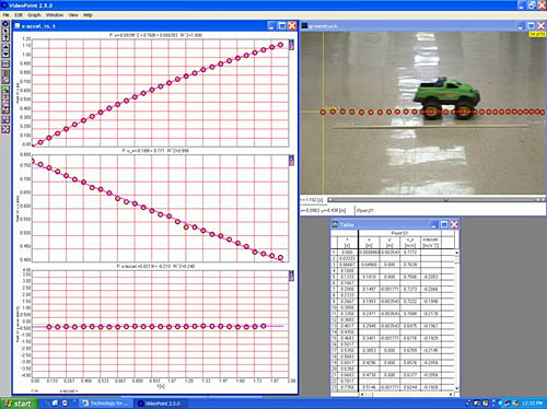
Figure 5. Screen shot of data collected using VideoPoint2.5.
While most simulations and other technologies take away the possibility for “experimental error,” students may incorporate error into video analysis via the “marking” process. Collected data can only be as accurate as students are in marking the exact same location on the moving object(s) in each frame. Although each frame is precisely timed by the digital recording, the exact position of the object at those times is dependent upon the marking skill of the student. The quality of the video is also a factor in marking errors. The faster the object is moving, the less distinctly it may appear in each frame. While this does not usually lead to as much error as is normally found in other timing and position measuring techniques, the introduction of error does make this form of analysis more realistic as a scientific process than do many simulations.
Digital video analysis represents one of the most recent and powerful technological innovations and has yet to be the subject of detailed research on its effectiveness as an instructional technique. Although the research on this form of technology is presently limited, a few studies related to video use have been conducted. Interactive digital video has been found to have a positive effect on students’ feelings of comfort in using computers (Escalada & Zollman, 1997). Another study found that the use of videotapes to introduce physics laboratory experiments had positive effects on student attitudes, but no effect on student achievement (Lewis, 1995). This study, however, was conducted before recent innovations in video analysis have made possible easier and more detailed analysis processes.
Other studies related to the use of probes/sensors and spreadsheet manipulation of data may also be applicable to video analysis. Once the video is marked, students have capabilities of viewing the video in real-time and watching the graphs respond in real-time to the motion of the object, leading to many of the same benefits that real-time MBL analyses provide. The further benefit of being able to analyze situations in ways that would not otherwise be possible also makes this technology an essential addition to any physics learning environment.
Computer Simulations Requiring Graphics
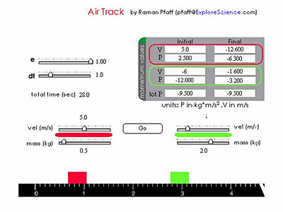
Figure 6. Air Track computer simulation.
One increasingly abundant form of technology available for students studying physics is the use of ready-made conceptual and phenomenological computer simulations and/or models of physical events. The NSTA (1999) recommended that to be effective, “simulation software should provide opportunities to explore concepts and models which are not readily accessible in the laboratory” (Declarations, ¶ 2). When cost, safety, time, or other issues are prohibiting factors, simulations can also “make it possible to explore physical situations where conducting the real experiment is impractical or impossible” (Steinberg, 2000, p. s37). These simulations may include various levels of interactivity, but most often involve dynamic motion that models the real event. Computer simulations are being used to “establish a cognitive framework or structure to accommodate further learning in a related subject area” and to “provide an opportunity for reinforcing, integrating and extending previously learned material” (Brant, Hooper, & Sugrue, 1991, p. 469).
An example of a computer simulation that can be used by students to quickly manipulate variables and gather data with greater detail and ease than would be possible using only physical equipment is the Web-based air track simulation accessed through the mechanics link at http://host.explorelearning.com/ESClassic/interact.htm (Figure 6). Initial conditions such as mass, velocity, and degree of elasticity may be specified. After the collision, final velocities and momenta are displayed.
Like all computer simulations, this simulated air track has limitations. The masses of the colliding objects may be specified only in the range of 0.2 to 3.0 kg, making it impossible to simulate a collision between two objects of greatly differing masses. The initial speed of each object may be at most 10 m/s, making it impossible to simulate collisions among objects with greatly differing speeds. The display of momenta values is a useful feature of this simulation, but there is no similar display of kinetic energies, making it difficult for students to readily examine changes in kinetic energies as the elasticity of the collision is manipulated.
An abundant resource of computer simulations available to physics teachers and currently used throughout the world is Physlets® developed by Wolfgang Christian and Davidson College (Figure 7).
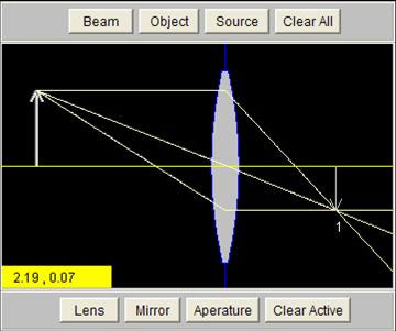
Figure 7. Physlets® example.
These simple Java applets may be downloaded and used for nonprofit educational purposes without requesting permission from Davidson College. Applets have been developed covering virtually all areas of physics concepts, including motion in one and two dimensions, forces, thermodynamics (Cox, Belloni, Dancy, & Christian, 2003), waves, sound, optics (Dancy, Christian, & Belloni, 2002), electricity, magnetism, relativity (Belloni, Christian, & Dancy, 2004), and quantum mechanics (Belloni & Christian, 2003).
The use of computer simulations has the potential for enormous benefits to student understanding of physics concepts. “Some scholars assert that simulations and computer-based models are the most powerful resources for the advancement and application of mathematics and science since the origins of mathematical modeling during the Renaissance” (Bransford, Brown, & Cocking, 2000, p. 215). Despite this potential, research into its instructional effectiveness has yielded inconsistent results. For example, although simulations have been shown to increase student understanding in areas of kinematics (Grayson & McDermott, 1996; Hewson, 1985) and optics (Goldberg, 1997), an early study by Cherryholmes (1966) reviewed “six studies and concluded that, except for heightened interest, no substantial evidence could be found to support claims that simulations produce greater cognitive gains and affective changes than other methods of instruction” (Brant et al., 1991, p. 469).
It is likely that the increased sophistication and realism of simulations available today may lead to different results if similarly conducted studies were performed again. In fact, a recently developed collection of computer simulations freely available from the World Wide Web is Physics Education Technology, or PhET (Perkins et al., 2006; Wieman & Perkins, 2005), has been the subject of more recent research. This research on the effectiveness of these computer simulations found that “students who used computer simulations in lieu of real equipment performed better on conceptual questions related to simple circuits, and developed a greater facility at manipulating real components” (Finkelstein et al., 2005).
The ineffectiveness of a computer simulation may not be the result of a poorly designed simulation. Brant et al. (1991) attributed the ineffectiveness of computer simulations to inappropriate instructional roles for which simulations are used. One problem is that “the use of computer simulations in classrooms is often reduced to step-by-step cookbook approaches, prescribed by teachers for students to follow” (Windschitl & Andre, 1998, p. 148). Used as such, a computer simulation shows no more promise for facilitating conceptual understanding than any other teacher directed activity. Brant et al. (1991) also found that “the effectiveness of the simulation is dependent upon the sequence of presentation of learning activities to students” (p. 477) and that the “optimal placement of the simulation in the instructional sequence seems to depend on the complexity of the subject matter and the purpose of instruction” (p. 479). Steinberg (2000) also contended that “the impact of using a simulation depends on the details of the program and the way in which it is implemented” (p. s37). As with any tool, its proper use in the right situations for the right purposes determines its value.
Even when simulations are used properly, a caution remains that although “simulations are extremely useful pedagogical tools, they are not experiments, and are thus of only limited utility as substitutes for actual laboratories” (McKinney, 1997, p. 591). One danger with using computer simulations is that “students will see no need to take responsibility for their own understanding, to verify, or to challenge” and “can result in students learning science passively” (Steinberg, 2000, p. s39). Other concerns voiced by Chinn and Malhotra (2002) are that because computer simulations are programmed in advance with causal variables, the “messiness of the natural world is artificially cleaned up” (p. 208) and “students may not learn to control variables in situations where they are not presented with a priori lists of variables” (p. 209).
It is important when using a simulation that the instructor helps students realize and critically evaluate the assumptions upon which the simulation program is written. Boulter and Buckley (2000) echoed these sentiments with their claim that students “often confuse the simplified, incomplete, and decontextualized models presented with the phenomena themselves” and fail to “understand the nature of the relationship between phenomena and their representations in models” (p. 42). Some students may actually believe that positive and negative signs actually exist in atoms and move around in an object. Students are not always aware that simulations may be programmed to do anything imaginable, even if it is not phenomenally accurate.
Research/Reference/Presentation Programs for Gathering, Reporting, and Displaying Information
Although computers may be used for many purposes, “the most prevalent use of computers in schools is for word processing” (Rios & Madhavan, 2000, p. 96). Programs such as the widely used Microsoft Word make it easy for data and information obtained from other sources to be pasted into a research document. Other research/reference/presentation programs used for reporting and/or displaying information include slideshow programs such as Microsoft PowerPoint, spreadsheet programs such as Microsoft Excel, and Web page programs such as Microsoft Front Page.
In studying student perceptions of slideshow presentations in large group instruction, Cassady (1998) determined that computer-aided presentations were superior to traditional lecture instruction in the following areas: “1) ability to hold the attention of the class, 2) interesting nature of material, 3) organization of material, 4) instructor preparedness, 5) ease in following the presentation, 6) clarity of information, and 7) flow of the information in the presentation” (p. 185). This study, however, attempted no measure of student achievement and cautioned that possibly the “inflated ratings of the computer-aided presentations arose due to novelty” (p. 186). The organizational qualities and ability to seamlessly integrate other forms of instructional methods (e.g., simulations, video clips, pictures, and graphics) make this a most valuable asset for large group presentations. Several presentations of physics topics may be found on the web site for the Center for Math and Science Education at Texas A & M University: http://www.science.tamu.edu/CMSE/powerpoint/index.asp.
Spreadsheets are currently used in physics instruction in a number of ways. According to the NSTA (1999) position statement, “Databases and spreadsheets should be used to facilitate the analysis of data via their organizational and visual representation capabilities” (Declarations, ¶ 4). The most common use is for simple display of data in graphical form. In addition to displaying data, spreadsheets have the capability of providing a “best fit” equation for the plotted points. A sampling of other more sophisticated uses of spreadsheets include programming for simulations in electrical circuit analysis (Kellogg, 1993; Silva, 1994), planetary orbits (Bridges, 1995), double slit interference (Field, 1995), and the Compton effect (Kinderman, 1992).
The World Wide Web is also an abundant source of information when investigating physics concepts. Many Web sites now contain physics tutorials with varying degrees of interactivity. In addition to its “round the clock” availability at no charge to the user, another advantage of this form of technology is that students with Internet access may work through these tutorials at their own pace outside of school as often as they like. These tutorials often include both text and simulations and may even include diagnostic self-assessment tools. Popular tutorial sites include the University of Colorado’s Physics 2000, The Physics Classroom, Fear of Physics, ThinkQuest’s Visual Physics, and for a small registration fee, Paul Hewitt’s Physics Place.
Successful Implementation of Technology
The mere presence of technology does not guarantee student learning, nor does the implementation of innovative practices (Coleman, Holcomb, & Rigden, 1998). In fact, according to Mottmann’s (1999, p. 76) review of literature, “there are no measurable differences in the physics knowledge gained when comparing reform and traditional methods of teaching.” Such claims are probably more an indication of the manner in which the technology or innovative practices were implemented than an indictment on the quality or usefulness of the product. Student learning will be maximized only when the instructional practices “are designed according to different educational and psychological theories and principles” (Schacter & Fagano, 1999, p. 339) in relation to individual students’ needs and abilities. Additionally, the effectiveness of computer technology depends not only on the way in which the computer and software are used, but also on the interactions of the students as they use the technology (Otero et al., 1999).
Regardless of the type of technology used,
the process of learning in the classroom can become significantly richer as students have access to new and different types of information, can manipulate it on the computer through graphic displays or controlled experiments in ways never before possible, and can communicate their results and conclusions in a variety of media to their teacher, students in the next classroom, or students around the world. (United States Department of Education, 1996, Benefits of technology use, ¶5)
One of the best ways to facilitate learning when using technology or other innovations is to construct the learning environment in accordance with the Bransford model of How People Learn (Bransford et al. 2000). According to this model, effective learning environments must be simultaneously “learner-centered” (p. 23), “knowledge-centered” (p. 24), “assessment-centered” (p. 24), and “community-centered” (p. 25). Using this model, developers of effective learning environments must take into consideration the unique characteristics of the individual learners and the processes through which they learn best, must conduct formative assessments, and must establish support for a community of learners. The research related to student achievement in technology-rich environments serves as support for each of these effective learning environment characteristics. Effectiveness of technology implementation is, therefore, dependent upon the same features that make any instructional practice effective.
References
Beichner, R. (1990). The impact of video motion analysis on kinematics graph interpretation skills. AAPT Announcer, 26, 86.
Belloni, M., & Christian, W. (2003). Physlets® for quantum mechanics. Computing in Science and Engineering, 5(1), 90-96.
Belloni, M., Christian, W., & Dancy, M. (2004). Teaching special relativity using Physlets®, The Physics Teacher, 42(5), 284-290.
Boulter, C., & Buckley, B. (2000). Constructing a typology of models for science education. In J. Gilbert & C. Boulter (Eds.), Developing models in science education (pp. 41-57). The Netherlands: Kluwer Academic Publishers.
Bransford, J., Brown, A., & Cocking, R. (Eds.). (2000). How people learn: Brain, mind, experience, and school. Washington: National Academy Press.
Brant, G., Hooper, E., & Sugrue, B. (1991). Which comes first, the simulation or the lecture? Journal of Educational Computing Research, 7(4), 469-481.
Brasell, H. (1987). The effect of real-time laboratory graphing on learning graphic representations of distance and velocity. Journal of Research in Science Teaching, 24(4), 385-395.
Bridges, R. (1995). Fitting planetary orbits with a spreadsheet. Physics Education, 30(5), 266-271.
Brungardt, J., & Zollman, D. (1995). The influence of interactive videodisc instruction using real-time analysis on kinematics graphing skills of high school physics students. Journal of Research in Science Teaching, 32(8), 855-869.
Bryan, J. (2004). Video analysis software and the investigation of the conservation of mechanical energy. Contemporary Issues in Technology and Teacher Education [Online serial], 4(3). Retrieved March 20, 2006, from https://citejournal.org/vol4/iss3/science/article1.cfm.
Bryan, J. (2005). Video analysis: Real-world explorations for secondary mathematics. Learning and Leading with Technology, 32(6), 22-24.
Cassady, J. (1998). Student and instructor perceptions of the efficacy of computer-aided lecutres in undergraduate university courses. Journal of Educational Computing Research, 19(2), 175-189.
Cherryholmes, C. (1966). Some current research on effectiveness of educational simulation: Implications for alternative strategies. The American Behavioral Scientist, 10, 4-7.
Chinn, C., & Malhotra, B. (2002). Epistemologically authentic inquiry in schools: A theoretical framework for evaluating inquiry tasks. Science Education, 86, 175-218.
Coleman, A., Holcomb, D., & Rigden, J. (1998). The Introductory Physics Project 1987-1995: What has it accomplished? American Journal of Physics, 66, 212-224.
Cox, A., Belloni, M., Dancy, M., & Christian, W. (2003). Teaching thermodynamics with Physlets® in introductory physics. Physics Education, 38(5), 433-440.
Dancy, M., Christian, W., & Belloni, M. (2002). Teaching with Physlets®: Examples from optics. The Physics Teacher, 40(8), 494-499.
Escalada, L., & Zollman, D. (1997). An investigation on the effects of using interactive digital video in a physics classroom on student learning and attitudes. Journal of Research in Science Teaching, 34(5), 467-489.
Field, R. (1995). A spreadsheet simulation for a Young’s double slits experiment. Physics Education, 30(4), 230-235.
Finkelstein, N., Adams, W., Keller, C., Kohl, P., Perkins, K., Podolefsky, N., Reid, S., & LeMaster, R. (2005). When learning about the real world is better done virtually: A study of substituting computer simulations for laboratory equipment. Physical Review Special Topics – Physics Education Research, 1(1), 010103.
Flick, L. & Bell, R. (2000). Preparing tomorrow’s science teachers to use technology: Guidelines for science educators. Contemporary Issues in Technology and Teacher Education, 1(1), 39-60.
Garofalo, J., Drier, S., Harper, S., Timmerman, M., & Shockey, T. (2000). Promoting appropriate uses of technology in mathematics teacher preparation. Contemporary Issues in Technology and Teacher Education, 1(1), 66-88.
Gilbert, J., Boulter, C., & Elmer, R. (2000). Positioning models in science education and in design and technology education. In J. Gilbert & C. Boulter (Eds.), Developing models in science education (pp. 3-17). The Netherlands: Kluwer Academic Publishers.
Goldberg, F. (1997). Constructing physics understanding in a computer-supported environment. American Institute of Physics Conference Proceedings, 399, 903-911.
Graham, T., & Rowlands, S. (2000). Using computer software in the teaching of mechanics. International Journal of Mathematical Education in Science and Technology, 31(4), 479-493.
Grayson, D., & McDermott, L. (1996). Use of the computer for research on student thinking in physics. American Journal of Physics, 64, 557-565.
Hasson, B., & Bug, A. (1995). Hands-on and computer simulations. The Physics Teacher, 33, 230-236.
Hewson, P. (1985). Diagnosis and remediation of an alternate conception of velocity using a microcomputer program. American Journal of Physics, 53, 684-690.
Kellogg, D. (1993). Spreadsheet circuitry. Science Teacher, 60(8), 21-23.
Kinderman, J. (1992), Investigating the Compton effect with a spreadsheet. The Physics Teacher, 30(7), 426-428.
Lederman, N., & Niess, M. (2000). Technology for technology’s sake or for the improvement of teaching and learning? School Science and Mathematics, 100(7), 345-348.
Lewis, R. (1995). Video introductions to the laboratory: Students positive, grades unchanged. American Journal of Physics, 63(5), 468-470.
McKinney, W. (1997). The educational use of computer based science simulations: Some lessons from the philosophy of science. Science and Education, 6, 591-603.
Mottmann, J. (1999). Innovations in physics teaching. The Physics Teacher, 37, 74-77.
National Science Teachers Association. (1990). Science teachers speak out: The NSTA lead paper on science and technology education for the 21st century. Washington, DC: Author.
National Science Teachers Association. (1999). NSTA Position Statement: The use of computers in science education. Retrieved March 20, 2006, from http://www.nsta.org/159&psid=4
Otero, V., Johnson, A., & Goldberg, F. (1999). How does the computer facilitate the development of physics knowledge by prospective elementary teachers? Journal of Education, 181(2), 57-89.
Perkins, K., Adams, W., Dubson, M., Finkelstein, N., Reid, S., Wieman, C., & LeMaster, R. (2006). PhET: Interactive simulations for teaching and learning physics. The Physics Teacher, 44(1), 18-23.
Rios, J., & Madhavan, S. (2000). Guide to adopting technology in the physics classroom. The Physics Teacher, 38, 94-97.
Schacter, J., & Fagano, C. (1999). Does computer technology improve student learning and achievement? How, when, and under what conditions? Journal of Educational Computing Research, 20(4), 329-343.
Silva, A. (1994). Simulating electrical circuits with an electronic spreadsheet. Computers and Education, 22(4), 345-353.
Steinberg, R. (2000). Computers in teaching science: To simulate or not to simulate? American Journal of Physics Supplement, 68(s7), s37-s41.
Steinberg, M., & Wainwright, C. (1993). Using models to teach electricity – The CASTLE project. The Physics Teacher, 31, 353-357.
Thornton, R., & Sokoloff, D. (1990). Learning motion concepts using real-time microcomputer- based laboratory tools. American Journal of Physics, 58, 858-867.
United States Department of Education. (1996). Getting America’s students ready for the 21st century: Meeting the technology literacy challenge – A report to the nation on technology and education . Retrieved April 18, 2006, from http://www.ed.gov/about/offices/list/os/technology/plan/national/index.html
Wieman, C., & Perkins, K. (2005). Transforming physics education, Physics Today, 58(11), 36.
Windschitl, M., & Andre, T. (1998). Using computer simulations to enhance conceptual change: The roles of constructivist instruction and student epistemological beliefs. Journal of Research in Science Teaching, 35(2), 145-160.
Technology Resources
DataPoint – http://www.stchas.edu/faculty/gcarlson/physics/datapoint.htm
Fear of Physics – http://www.fearofphysics.com/
Interactive Physics – http://www.interactivephysics.com/
LoggerPro – http://www.vernier.com/soft/lp.html
Measurement-in-Motion – http://www.learn.motion.com/products/measurement/index.html
NetLogo – http://ccl.northwestern.edu/netlogo/
Physics 2000 – http://www.colorado.edu/physics/2000/index.pl
Physics Education Technology – http://www.colorado.edu/physics/phet/web-pages/index.html
Physics Place – http://occawlonline.pearsoned.com/sms_files/physicsplace/login. html
Physics ToolKit (formerly known as World-in-Motion) – http://www.physicstoolkit.com/
PowerPoint Physics – http://www.science.tamu.edu/CMSE/powerpoint/index.asp.
Physlets® – http://webphysics.davidson.edu/Applets/Applets.html
STELLA – http://www.iseesystems.com/softwares/Education/StellaSoftware.aspx
The Physics Classroom – http://www.physicsclassroom.com/
Tracker – http://www.cabrillo.edu/~dbrown/tracker/index.html
VideoPoint – http://www.lsw.com/videopoint/
Visual Physics – http://library.thinkquest.org/10170/main.htm
Author Info
Joel Bryan
Texas A&M University
[email protected]
![]()