National standards for mathematics and science teaching and learning currently emphasize the use of technology in mathematics and science courses in order to facilitate the development of a “technologically literate” society that is prepared to be productive in today’s technology-dependent society. The National Science Teachers Association (NSTA) position statement on the use of computers in science education states plainly that “computers should have a major role in the teaching and learning of science” (NSTA, 1999, ¶1) and emphasize technology’s use for data collection, manipulation, and presentation. According to the Technology Principle stated in the National Council of Teachers of Mathematics (NCTM, 2000) Principles and Standards for School Mathematics, “electronic technologies…are essential tools for teaching, learning, and doing mathematics” because “they furnish visual images of mathematical ideas, they facilitate organizing and analyzing data, and they compute efficiently and accurately” (p. 24). These same standards further call for making mathematics and science relevant to learners. Making the connections between what is studied in class and what is experienced in life outside of the classroom leads to a more developed and deeper understanding of the concepts (Boaler, 1998; Borenstein, 1997). Because technology has rapidly become a part of people’s everyday experiences in life outside of the classroom, its use in the classroom serves as an excellent means for helping educators meet the relevancy objectives.
If technology use and real world applications of concepts are desired in our nation’s mathematics and science classrooms, then courses that prepare future teachers of these subjects should incorporate and model effective uses of each of these. According to Flick and Bell’s (2000) guidelines for technology use in science teacher preparation, “technology should be introduced in the context of science content,” “technology instruction in science should take advantage of the unique features of technology,” and “technology should make science views more accessible” (p. 40). Similar to this are Garofalo, Drier, Harper, Timmerman, and Shockey’s (2000) guidelines for technology use in mathematics teacher preparation. Among other things, they too contend that instructors should “introduce technology in context” (p. 67) and that technology should be used to “extend beyond or significantly enhance what could be done without technology” (p. 71). As a general rule, technology should be used when it allows one to either do something that could not be done at all without it or to do something better than could be done without it.
Although much of the focus on the use of technology in mathematics and science has centered on the use of graphing calculators (Adie, 1998; Embse & Engebretsen, 1996; Korithoski, 1996), computer-based laboratory sensors (Lapp & Cyrus, 2000; Thornton & Sokoloff, 1990), and computer simulations (Wilkinson, 1995), another more recently developed and relatively inexpensive technology meets each of these criteria and provides an excellent opportunity for preservice science and mathematics teacher content and/or pedagogy courses to model investigations that are greatly enhanced through technology use. By using inexpensive video analysis software and movie clips, students can now quickly and efficiently gather data from real-world situations, which can then be manipulated, analyzed, and graphed in ways and with ease not always so accessible with those other forms of technology.
Examples of Currently Available Video Analysis Programs
A number of relatively inexpensive video analysis programs are currently available, including VideoPoint (which is promoted by the American Association of Physics Teachers), Physics ToolKit (formerly known as World-in-Motion), and Measurement-in-Motion. Increasing interest in this type of technology and the awareness of its potential for enhancing student learning has led makers of calculator-based software and probes, such as Vernier’s LoggerPro, to incorporate similar video analysis capabilities into the latest upgrades of their existing programs.
Not only do these video analysis programs come prepackaged with video clips that are ready to be analyzed, they also allow users to import and analyze video clips from other sources, including movies produced by students in the laboratory setting immediately before analysis. Of these programs, VideoPoint has the most sophisticated features and is perhaps the most versatile, although Physics ToolKit may be the most cost effective. Users of this software may find, as I did, that the video clips contained in the Physics ToolKit program are more suitable for introductory level physics investigations than those contained in VideoPoint. However, VideoPoint also functions as a video capture program, allowing users to easily make movies in the lab setting for immediate use with the analysis program. Macintosh users may prefer Measurement-in-Motion. It was originally designed for exclusive use with Macintosh computers, but it has recently become available for use with Windows-based personal computers.
The feature common to these and other video analysis programs is that the computer mouse cursor is used to “mark” the position of an object in each frame of a video clip. Users most likely will then instruct the software to convert pixel locations to more applicable position units and, generally, also have the option to translate and rotate the coordinate axes to meet the parameters of the specific phenomena being investigated. With just a click of the mouse button, the software program will then take the position data and make relevant calculations necessary to produce informative graphs. Position, velocity, acceleration, force, momentum, and energy graphs, among others, can all be quickly produced and graphed. Most of the video analysis programs also have the capability for computing and reporting “best fit” equations for these curves.
A free software program called Tracker contains many of the same features contained in the previously described commercial programs. Users “mark” video frames, set the origin to the desired location, and calibrate the video for real-world measurement values. Tracker then calculates motion values, constructs graphs, and draws and manipulates force, velocity, and acceleration vectors. The Tracker Web page contains links to tutorials and several video clips ready for analysis. Tracker also has the capability of creating a line profile tool that measures the brightness of the image pixels it lies on in order to generate spectral line profiles and analyze diffraction and interference patterns, a feature not currently available with other video analysis programs.
Another free software program, called DataPoint, is available, but it requires students to import the marked data into a spreadsheet and then manipulate it to produce the relevant information. Although this program is copyrighted, its developer allows it to be downloaded from his Web site free of charge. He does ask that users notify him that they are using the software and let him know how it serves their needs and how it can be improved. In order to obtain more meaningful results, students using this program will need to convert their data sets, which contain x and y pixel positions of the location of the object with time, to appropriate position units using proportions and a known measurement standard. Users may also need to make linear translation manipulations to move the origins to desired locations. The use of a more “bare bones” program such as this may be preferred if the instructor desires that students have more responsibility for manipulating data and generating velocities and accelerations from position changes.
A video analysis informational page linked to the Texas A&M University Center for Mathematics and Science Education Web site contains 19 short video clips that may be downloaded and analyzed in any of these programs. Also linked to this Web site are instructional videos demonstrating the use of VideoPoint, DataPoint, and the Microsoft Excel spreadsheet program for data analysis, along with suggestions for the use of each video clip.
A VideoPoint Investigation of a Bouncing Ball’s Conservation of Mechanical Energy
Introductory level physics courses typically present rising and/or falling objects as one example of the conservation of mechanical energy. Instructors and textbooks typically inform students that after a ball is tossed upward, it loses kinetic energy (KE = 0.5mv2, where m = the mass of the object and v = the speed of the object) and gains gravitational potential energy (PEg = mgh, where m = the mass of the object, g = the gravitational acceleration value of 9.8 m/s/s, and h = the height above the arbitrarily chosen zero position) as it rises; and then loses gravitational potential energy and gains kinetic energy as it falls, such that the total mechanical energy (TE = KE + PEg) remains constant at every location during the trip. Seldom do the students or instructor perform any actual measurement-based calculations of the energies involved, except for using the maximum height above the arbitrarily chosen zero position of the ball before release to determine its maximum gravitational potential energy.
Since the stationary ball’s kinetic energy at this maximum height is known by direct observation to be 0, the total mechanical energy of the ball at any location is, therefore, equal to its maximum gravitational potential energy. Although students will predictably use the mechanical energy conservation relationship (TE = KE + PEg) to specify the amounts of kinetic and gravitational potential energies at any location of the ball’s path, they rarely collect any actual data to support these calculations.
Inexpensive video analysis technologies now make possible a more detailed investigation of the conservation of energy involved in this and many other situations. By using this technology, students not only generate actual data supporting claims of energy conservation for a rising and falling ball, they may also investigate the loss of mechanical energy during bouncing and the changes in the velocity, acceleration, and net force on the ball at any location of its movement.
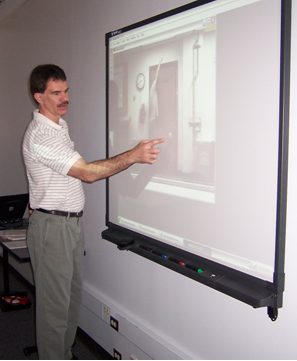
Figure 1. PHYS 205 instructor demonstrates the use of VideoPoint at the SMART Board.
Preservice teachers taking a conceptual physics course (PHYS 205) designed for middle grades science and mathematics specialists at Texas A&M University used VideoPoint video analysis software to gather data in order to analyze this and three other motion situations. For these four video analysis activities, students met in the College of Education and Human Development’s Verizon Interactive Classroon (VIC), a state of the art “classroom of the future” that was constructed through funding obtained from the Verizon Foundation. Contained in the VIC were moveable tables/work stations with wireless laptop computers having compact disk burning capabilities, an LCD projector, and a SMART Board interactive white board to aid in instructional delivery. The instructor’s use of the SMART Board to demonstrate the capabilities of VideoPoint is shown in Figure 1.
To begin the activity, the actual ball present in the soon-to-be analyzed video clip was dropped as a demonstration, and students were asked to describe the changes in the falling ball’s energies. Although most all students will correctly state that while the ball falls, its total energy remains constant as it loses potential energy and gains kinetic energy, it is generally unknown whether or not these students have a deeper understanding of this situation, and if they can correctly predict the graphical representation of the energies involved. Therefore, as a prelab investigation, students first made predictive sketches of what they expected graphs of potential, kinetic, and total energies to look like as a ball falls and also as a ball falls and bounces four times.
An examination of the predictions handed in by the 27 pairs of spring 2004 Physics 205 students prior to this laboratory activity confirmed that, although most students generally said the correct words, they often failed to develop an acceptable conceptual understanding or were unable to predict how those ideas would be displayed graphically. Only one group failed to hand in a prediction that displayed a decrease in potential energy and a simultaneous increase in kinetic energy. However, despite having previously performed several laboratory activities in which they generated quadratic curves for accelerated motion, 15 of these 26 pairs (57.7%) displayed linear, instead of quadratic, changes (Figure 2) in their energy graphs. More surprisingly, 15 of the 27 pairs (55.6%) of students represented their constant total energy by a line passing through the intersection of the kinetic and potential energy curves, an occurrence which is also indicated in Figure 2. This inability to relate actual motion to its graphical representations, despite being able to correctly articulate the description of the motion, has been studied and described in numerous reports (Beichner, 1994, 1996, 1999; McDermott, Rosenquist, & van Zee, 1987).
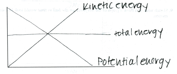 Figure 2. Sample energy graph I.
Only 2 of the 27 pairs (7.4%) of students handed in predictions corresponding to the acceptable representations of the energy graphs, one of which is shown in Figure 3.
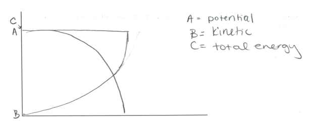 Figure 3. Sample energy graph II.
After completing their predictions, the pairs of students (Figure 4) used the VideoPoint program to open a video showing the 302-gram minibasketball falling and bouncing four times after being held and released by the instructor.
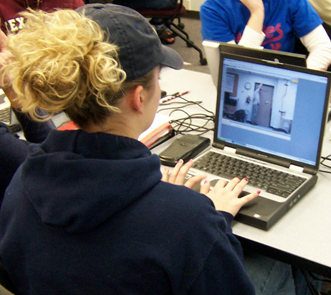 Figure 4. Preservice teachers using VideoPoint in Texas A&M’s VIC.
Since most digital video cameras film at a rate of approximately 29.97 frames/second, students were able to collect data describing precise locations of the ball every 1/30 sec. VideoPoint allowed students to “mark” the location of the ball in each of the 95 frames of this movie clip, resulting in the movie window shown in Figure 5. “Marking” the frames of the video clip was done by simply moving the mouse cursor over the ball’s location in the frame and “clicking.” The program advanced the video clip automatically to the next frame, and even allowed the students to predetermine whether or not each frame of the movie was to be “marked,” that is, the students could set the program to advance to every second, third, fourth, fifth, etc….frame, a feature which is particularly useful when analyzing lengthy video clips. As each frame was “marked,” the vertical and horizontal positions of the ball at that precise time were entered into a data table and were available for viewing by the students when desired.
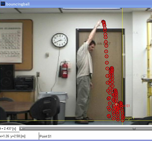
Figure 5. VideoPoint screenshot of “marked” video.
After marking each of the desired video frames, students quickly and easily moved the origin to the lowest marked position of the ball, used the meter stick in the video’s background for the scaling purpose of converting coordinates values from pixels to meters, and entered the mass of the ball, which was necessary for energy and force calculations. Although the video did indicate some horizontal movement by the ball, it was irrelevant to this analysis and, therefore, ignored. Students then used VideoPoint to produce informative graphs of the ball’s motion. Position, velocity, and acceleration graphs of the ball’s vertical motion with time are shown in Figure 6.
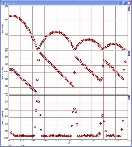
Figure 6. VideoPoint position, velocity, and acceleration graphs of a bouncing ball.
These three graphs contain a wealth of information that cannot be as easily obtained when using other data collection methods. Among other things, the position graph indicates the vertical position of the ball as it changes with time. The decreasing “width” of each parabolic section indicates the decreasing amount of time the ball was in the air between bounces. The decreasing height of each parabolic section indicates that the ball did not rise as high after a bounce.
One of the more interesting aspects of the velocity graph is that the “gaps” between each segment indicate the abrupt change in sign and direction of the ball as it bounces. Each of these segments cross the horizontal axis at the highest position of the ball and have slopes (not shown, but could be easily calculated) approximately equal to the accepted gravitational acceleration value (g = –9.8 m/s/s). The third graph, acceleration, not only displays the constant negative acceleration of the ball as it rises and falls, but also the brief but much greater positive acceleration during each bounce. The graph of the net force on the ball with time (Figure 7) indicates that the net force on the ball is a constant negative value corresponding to its weight (w = mg) as it both rises and falls, but is a much greater positive value during the brief time that the ball is in contact with the floor during a bounce.
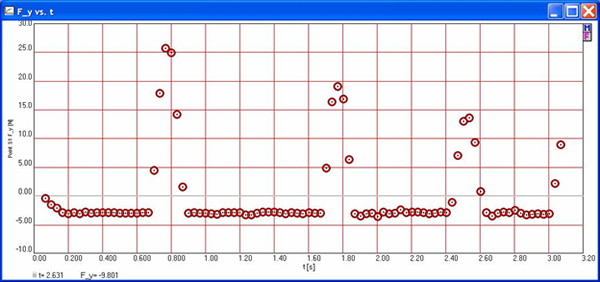
Figure 7. VideoPoint graph of the net force on the bouncing ball.
Students can further directly correlate the information contained in these and other graphs to the motion of the ball by viewing the graphs while playing the movie. As the movie plays, points on each graph are “highlighted” by the program in real time. Such a feature should provide similar benefits of “real time” graphing that make calculator-based laboratory (CBL) probes and software effective. Also, “clicking” on any point displayed in any graph will take the user to that precise frame in the movie.
If “a picture is worth a thousand words,” the energy graphs shown in Figure 8 embody a novel. By examining these graphs, my students readily saw verification that the sum total kinetic and gravitational potential energies remained constant as the ball rose and fell. Students also saw how the kinetic and gravitational potential energies increased and decreased inversely with each period of time in the air. This total mechanical energy decreased after each bounce, and its loss was indicated by the abrupt vertical “gaps” in the horizontal total energy segments. An inspection of the relative amount of mechanical energy lost in each bounce revealed that this ball conserved approximately 55-60% of its energy after each bounce. To conclude this exercise, students compared the actual graphs with their prelab predictions and developed lists of questions about each of the graphs that would be appropriate for classroom instruction.

Figure 8. VideoPoint graphs of kinetic, potential, and total energies of a falling ball.
On the exam covering concepts of work, power, and energy that was administered to these same students 2 full weeks after this video analysis laboratory investigation, one question asked students to sketch position, velocity, acceleration, and energy graphs depicting the motion of a “super ball” that would rise to 50% above its release point after each of four bounces. Although one cannot justifiably attribute success on this question as being solely dependent upon the use of the video analysis software, it is encouraging to note that not one single student in this class (n = 57) drew graphs having straight line segments for kinetic and gravitational potential energies and a total energy curve passing through their intersections as many had done in their prelab predictions. However, 6 students still drew a horizontal segment for total energy midway between the maximum and minimum kinetic/potential energy levels as before, and 7 others drew kinetic and potential energies with straight line segments.
Technology savvy physics teachers may readily call attention to the fact that similar results can be obtained in “real-time” using a microcomputer-based laboratory (MBL) motion sensor probe. The benefits of “real-time” graphing versus “delay-time” graphing are debatable. Although Brasell (1987) did find that “real-time” graphing with MBLs improved students’ graphing skills more so than “delay-time” graphing of the same events, a later study in which students analyzed motion contained on videotape showed no significant differences (Brungardt & Zollman, 1995). Graphing using today’s more sophisticated video analysis software, however, cannot be classified as the typical “delay-time” graphing, because once these programs have initially produced the graphs in delay-time, users then have the capability of viewing the action multiple times while following the graph in real-time.
Although it is true that some investigations may be made just as easily, accurately, and precisely using probeware and/or sensors, there are three important advantages of video analysis over probes and sensors.
- Video analysis allows for study of two-dimensional motion, such as revolving objects or projectiles.
- More than one object can be analyzed in any video, which can lead to detailed comparisons of multiple objects that are in the same system.
- Video analysis can be performed without all of the cumbersome wires and sensors associated with MBLs.
The versatility of video analysis is also an important feature. Any object(s) in any location that can be, or has been, videotaped can be analyzed. Computer technology today even makes possible the video analysis of any clip of motion “captured” from any available recording in videocassette (VHS), compact disk (CD), and digital video disk (DVD) formats.
Although computer simulations and other technologies, such as MBL probes and sensors, often take away the possibility for “experimental error” and raise concerns by Chinn and Malhotra (2002) that the “messiness of the natural world is artificially cleaned up” (p. 208) so that “students may not learn to control variables in situations where they are not presented with a priori lists of variables” (p. 209), students may introduce and encounter error using video analysis via the “marking” process. Collected data can only be as accurate as students are in marking the exact same location on the moving object(s) in each frame. Although each frame is precisely timed by the digital recording, the exact positions of the object(s) at those times are dependent upon the marking skill of the student.
The accuracy with which the distance scale for the motion is marked is also a possible source of error. If the known distance is marked too short, then all velocities and accelerations calculated by the program will be too large, with the opposite true if the scale is marked too large. The quality of the video is also a factor that influences marking errors. The faster the object is moving, the more “fuzzy” it may appear in each frame. While these error sources do not usually lead to as much error as is normally found in other timing and position measuring techniques, the introduction of error does make this form of analysis more realistic as a scientific process than do many simulations and MBL probes.
Because it is a relatively recent technological development, few studies have been conducted to examine the effectiveness of implementing video analysis as an instruction tool in either mathematics or science. Like Escalada and Zollman (1997), I have found that most of my students discovered the video analysis software relatively simple to learn and recognized its benefits in helping them learn physics.
A more recent study by Pappas, Koleza, Rizos, and Skordoulis (2002) did find that the VideoPoint video analysis program was successful in helping preservice teachers better understand the links between multiple representations of motion presented in graphical, tabular, and formula formats. In addition, video analysis software may be used for many of the same purposes currently served by MBL motion sensors and photogates. One can cautiously make assumptions that some of the same features that make MBLs effective, such as quickly generating graphs so that students may spend more of their time studying physics concepts instead of burdensome point plotting (Barton, 1998), should also lead to success using video analysis.
Video analysis technology has improved immensely since the seemingly ancient 20th century method of placing an overhead transparency on a television screen and marking the locations of some object during pause and advance with a videocassette player/recorder (VCR). Today’s higher quality digital video, which increases the number of coordinate points and allows for more precise study, causes many past studies on the effectiveness of video analysis instructional methodologies to be outdated or obsolete.
Therefore, many of the studies on the effectiveness of real-time and delayed-time graphing from the past 20 years will need to be replicated in order to see if and how recent technological advances have influenced the value of this instructional method. Furthermore, neither the use of video analysis software, other forms of technology, nor any innovative practices can guarantee that learning will be enhanced for the user (Coleman, Holcomb, & Rigden, 1998). The effectiveness of computer technology depends not only on the way in which the computer and software are used, but also on the interactions of the students as they use the technology (Otero, Johnson, & Goldberg, 1999).
Regardless of the type of computer technology or any other educational innovation used in physics instruction, student learning will be maximized only when the instructional practices “are designed according to different educational and psychological theories and principles” (Schacter & Fagano, 1999, p. 339) in relation to individual students’ needs and abilities. Research on the effectiveness of video analysis should occur in a variety of instructional methodologies, including but not limited to constructivism, guided and unguided inquiry, and direct instruction.
Conclusion
In addition to its obvious benefits for physics investigations, video analysis software can be an effective addition to mathematics instruction. According to NCTM standards,
The use of real-world problems to motivate and apply theory, the use of computer utilities to develop conceptual understanding, the connections among a problem situation, its model as a function in symbolic form, and the graph of that function, and functions that are constructed as models of real-world problems [are all] topics that should receive increased attention [in mathematics classes]. (Roth, 1992, p. 307)
The use of video analysis technology not only serves these functions, but also provides a cost and time effective means of bringing authentic investigations into mathematics classes and serves to meet the directives of the NCTM for incorporating technology into our teaching practices (NCTM, 2000; Rojano, 1996).
This emerging video analysis technology is rapidly changing how teaching and learning can occur in both science and mathematics classes. Software engineers are now developing programs similar to these that are compatible with portable handheld technologies, which should greatly increase the versatility of video analysis as an instruction method. Such products meet the most important guidelines for the appropriate use of technology in science and mathematics study, and the use of these products should be an element in courses for preservice science and mathematics teachers and in professional development sessions for in-service teachers.
Additionally, the development and use of computer laboratory facilities similar to the Verizon Interactive Classroom at Texas A&M serve not only as an instructional tool for science and mathematics content courses, but also provide a means for demonstrating appropriate pedagogical methods and building technological literacy in preservice teachers.
References
Adie, G. (1998). The impact of the graphics calculator on physics teaching. Physics Education, 33(1), 50-54.
Barton, R. (1998). Why do we ask pupils to plot graphs? Physics Education, 33(6), 366-367.
Beichner, R. (1994). Testing student interpretation of kinematics graphs. American Journal of Physics, 62(8), 750-762.
Beichner, R. (1996). Impact of video motion analysis on kinematics graph interpretation skills. American Journal of Physics, 64(10), 1272-1277.
Beichner, R. (1999). Video-based labs for introductory physics courses. Journal of College Science Teaching, 29(2), 101-104.
Boaler, J. (1998). Alternative approaches to teaching, learning and assessing mathematics. Evaluation and Program Planning, 21(2), 129-141.
Borenstein, M. (1997). Mathematics in the real world. Learning and Leading with Technology, 24(7), 34-39.
Brasell, H. (1987). The effect of real-time laboratory graphing on learning graphic representations of distance and velocity. Journal of Research in Science Teaching, 24(4), 385-395.
Brungardt, J., & Zollman, D. (1995). Influence of interactive videodisc instruction using simultaneous-time analysis on kinematics graphing skills of high school physics students. Journal of Research in Science Teaching, 32(8), 855-869.
Chinn, C., & Malhotra, B. (2002). Epistemologically authentic inquiry in schools: A theoretical framework for evaluating inquiry tasks. Science Education, 86, 175-218.
Coleman, A., Holcomb, D., & Rigden, J. (1998). The Introductory Physics Project 1987-1995: What has it accomplished? American Journal of Physics, 66(2), 212-224.
Embse, C., & Engebretsen, A. (1996). A mathematical look at a free throw using technology. Mathematics Teacher, 89(9), 774-779.
Escalada, L., & Zollman, D. (1997). An investigation on the effects of using interactive digital video in a physics classroom on student learning and attitudes. Journal of Research in Science Teaching, 34(5), 467-489.
Flick, L. & Bell, R. (2000). Preparing tomorrow’s science teachers to use technology: Guidelines for science educators. Contemporary Issues in Technology and Teacher Education, 1(1), 39-60.
Garofalo, J., Drier, H., Harper, S., Timmerman, M., & Shockey, T. (2000). Promoting appropriate uses of technology in mathematics teacher preparation. Contemporary Issues in Technology and Teacher Education, 1(1), 66-88.
Korithoski, T. (1996). Finding quadratic equations for real-life situations. Mathematics Teacher, 89(2), 154-157.
Lapp, D., & Cyrus, V. (2000). Using data-collection devices to enhance students’ understanding. Mathematics Teacher, 93(6), 504-510.
McDermott, L. C., Rosenquist, M. L., & van Zee, E. H. (1987). Student difficulties in connecting graphs and physics: Examples from kinematics. American Journal of Physics, 55(6), 503- 513.
National Council of Teachers of Mathematics. (2000). Principles and standards for school mathematics. Reston, VA: Author.
National Science Teachers Association. (1999). Position statement: The use of computers in science education. Retrieved February 5, 2004, from http://www.nsta.org/positionstatement&psid=4
Otero, V., Johnson, A., & Goldberg, F. (1999). How does the computer facilitate the development of physics knowledge by prospective elementary teachers? Journal of Education, 181(2), 57-89.
Pappas J., Koleza E., Rizos J., & Skordoulis, C. (2002, July). Using interactive digital video and motion analysis to bridge abstract mathematical notions with concrete everyday experiences. Paper presented at the 2nd International Conference on the Teaching of Mathematics, Hersonissos, Greece. Retrieved April 13, 2004, from http://www.math.uoc.gr/%7Eictm2/Proceedings/pap299.pdf
Rojano, T. (1996). Developing algebraic aspects of problem solving within a spreadsheet environment. In N. Bednarz, C. Kieran, & L. Lee (Eds.), Approaches to algebra: Perspectives for research and teaching. Boston: Kluwer Academic Publishers.
Roth, W. (1992). Bridging the gap between school and real life: Toward an integration of science, mathematics, and technology in the context of authentic practice. School Science and Mathematics, 92(6), 307-317.
Schacter, J., & Fagano, C. (1999). Does computer technology improve student learning and achievement? How, when, and under what conditions? Journal of Educational Computing Research, 20(4), 329-343.
Thornton, R., & Sokoloff, D. (1990). Learning motion concepts using real-time microcomputer-based laboratory tools. American Journal of Physics, 58(9), 858-857.
Wilkinson, L. (1995). Physics academic software: Graphs and tracks. The Physics Teacher, 33(4), 254-255.
Technology Resources
DataPoint – http://www.stchas.edu/faculty/gcarlson/physics/datapoint.htm
Measurement in Motion – http://www.learninginmotion.com/products/measurement/index.html
Physics Toolkit (formerly World-in-Motion) – http://members.aol.com/raacc/wim.html
SMART Board – http://www.smarttech.com/ads/smartcd/index.asp
Texas A&M’s Center for Mathematics and Science Education Video Analysis Web site – http://www.science.tamu.edu/CMSE/videoanalysis/index.asp
Tracker – http://www.cabrillo.edu/~dbrown/tracker/index.html
Verizon Foundation – http://foundation.verizon.com/
Vernier’s Logger Pro 3 – http://www.vernier.com/soft/lp.html
VideoPoint – http://www.lsw.com/videopoint/
Author Note:
Joel Bryan
Texas A&M University
[email protected]
![]()